This is the fourth post in a series documenting my adventures in creating a GPU path tracer from scratch
1.
Tracing Light in a Virtual World
2.
Creating Randomness and Accumulating Change
3.
Shooting Object from Across the Way
So we're finally here! We've learned everything we need to actually implement a path tracer! First off, let me apologize for taking so long to get this post up. Things started getting busy at work again and I was in a car accident last week. So I've been recovering from that. Also, the implementation I showed a picture of last post turned out to be mathematically incorrect. (The current simulation is still far from physically correct, but I'll get to that later in the post) But, that's in the past now; let's get started.
A Quick Review
Before we launch into the code. let's first go over what we're trying to do. For each pixel we want to simulate the light that bouces around the scene in order to calculate a color. This calculation can be described by the Rendering Equation:
\[L_{\text{o}}(p, \omega_{\text{o}}) = L_{e}(p, \omega_{\text{o}}) + \int_{\Omega} f(p, \omega_{\text{o}}, \omega_{\text{i}}) L_{\text{i}}(p, \omega_{\text{i}}) \left | \cos \theta_{\text{i}} \right | d\omega_{\text{i}} \]
Wow, that's looks intimidating. But once we break it down it's actually a pretty simple concept. In English, the equation is:
The outgoing light from a point equals the emmisive light from the point itself, plus all the incoming light attenuated by a function of the material (the BSDF) and the direction of the incoming light.
The integral is just a mathematical way of adding up all the incoming light coming from the hemisphere around the point.
That said, once you start taking into account light reflected off of things, being absorbed by things, being refracted by things, etc, things start to become very complex. For almost all scenes, this integral can not be analytically solved.
A very simple approximation of this integral is to only take into account the light that is directly coming from light sources. With this, the integral collapses into a simple sum over all the lights in the scene. Aka:
\[L_{\text{o}}(p, \omega_{\text{o}}) = L_{e}(p, \omega_{\text{o}}) + \sum_{k = 0}^{n} f(p, \omega_{\text{o}}, \omega_{\text{i}}) L_{\text{i, k}}(p, \omega_{\text{i}}) \left | \cos \theta_{\text{i}} \right |\]
This is what Direct Lighting Ray Tracers do. They shoot rays from the point to each light, and test for obscurance between them.
However, you can simplify it further by also ignoring the obscurance checks. That is, you light the pixel with the assumption that it is the only thing in the scene. This is exactly what most real-time renderers do. It is known as a
local lighting model. It's extremely fast because each pixel can be lit independently; the incoming light at the pixel is determined only by the lights in the scene, not on the scene itself. However, the speed comes at a cost. By disregarding the scene, you lose all global illumination effects. Aka, shadows, light bleeding, indirect light, specular reflections, etc. These have to be approximated using tricks and/or hacks. (Shadow mapping, light baking, screen space reflections, etc.)
Another way to approximate the integral is by using
Monte Carlo Integration.
\[\int f(x) \, dx \approx \frac{1}{N} \sum_{i=1}^N \frac{f(x_i)}{pdf(x_{i})}\]
It says that you can approximate an integral by averaging successive random samples from the function. As $N$ gets large, the approximation gets closer and closer to the solution. $pdf(x_{i})$ represents the
probability density function of each random sample.
Path tracing uses Monte Carlo Integration to solve the rendering equation. We sample by tracing randomly selected light paths around the scene.
The Path Tracing Kernel
I figure the best way to understand the path tracing algorithm is just to post the whole kernel, and then go over each line / function, explaining as we go. So here's the whole thing:
__global__ void PathTraceKernel(unsigned char *textureData, uint width, uint height, size_t pitch, DeviceCamera *g_camera, Scene::SceneObjects *g_sceneObjects, uint hashedFrameNumber) {
    // Create a local copy of the arguments
    DeviceCamera camera = *g_camera;
    Scene::SceneObjects sceneObjects = *g_sceneObjects;

    // Global threadId
    int threadId = (blockIdx.x + blockIdx.y * gridDim.x) * (blockDim.x * blockDim.y) + (threadIdx.y * blockDim.x) + threadIdx.x;

    // Create random number generator
    curandState randState;
    curand_init(hashedFrameNumber + threadId, 0, 0, &randState);


    int x = blockIdx.x * blockDim.x + threadIdx.x;
    int y = blockIdx.y * blockDim.y + threadIdx.y;

    // Calculate the first ray for this pixel
    Scene::Ray ray = {camera.Origin, CalculateRayDirectionFromPixel(x, y, width, height, camera, &randState)};


    float3 pixelColor = make_float3(0.0f, 0.0f, 0.0f);
    float3 accumulatedMaterialColor = make_float3(1.0f, 1.0f, 1.0f);

    // Bounce the ray around the scene
    for (uint bounces = 0; bounces < 10; ++bounces) {
        // Initialize the intersection variables
        float closestIntersection = FLT_MAX;
        float3 normal;
        Scene::LambertMaterial material;

        TestSceneIntersection(ray, sceneObjects, &closestIntersection, &normal, &material);

        // Find out if we hit anything
        if (closestIntersection < FLT_MAX) {
            // We hit an object

            // Add the emmisive light
            pixelColor += accumulatedMaterialColor * material.EmmisiveColor;


            // Shoot a new ray

            // Set the origin at the intersection point
            ray.Origin = ray.Origin + ray.Direction * closestIntersection;
            // Offset the origin to prevent self intersection
            ray.Origin += normal * 0.001f;

            // Choose the direction based on the material
            if (material.MaterialType == Scene::MATERIAL_TYPE_DIFFUSE) {
                ray.Direction = CreateUniformDirectionInHemisphere(normal, &randState);

                // Accumulate the diffuse color
                accumulatedMaterialColor *= material.MainColor /* * (1 / PI)  <- this cancels with the PI in the pdf */ * dot(ray.Direction, normal);

                // Divide by the pdf
                accumulatedMaterialColor *= 2.0f; // pdf == 1 / (2 * PI)
            } else if (material.MaterialType == Scene::MATERIAL_TYPE_SPECULAR) {
                ray.Direction = reflect(ray.Direction, normal);

                // Accumulate the specular color
                accumulatedMaterialColor *= material.MainColor;
            }


            // Russian Roulette
            if (bounces > 3) {
                float p = max(accumulatedMaterialColor.x, max(accumulatedMaterialColor.y, accumulatedMaterialColor.z));
                if (curand_uniform(&randState) > p) {
                    break;
                }
                accumulatedMaterialColor *= 1 / p;
            }
        } else {
            // We didn't hit anything, return the sky color
            pixelColor += accumulatedMaterialColor * make_float3(0.846f, 0.933f, 0.949f);

            break;
        }
    }


    if (x < width && y < height) {
        // Get a pointer to the pixel at (x,y)
        float *pixel = (float *)(textureData + y * pitch) + 4 /*RGBA*/ * x;

        // Write pixel data
        pixel[0] += pixelColor.x;
        pixel[1] += pixelColor.y;
        pixel[2] += pixelColor.z;
        // Ignore alpha, since it's hardcoded to 1.0f in the display
        // We have to use a RGBA format since CUDA-DirectX interop doesn't support R32G32B32_FLOAT
    }
}
Initializing all the Variables
// Create a local copy of the arguments
DeviceCamera camera = *g_camera;
Scene::SceneObjects sceneObjects = *g_sceneObjects;

// Global threadId
int threadId = (blockIdx.x + blockIdx.y * gridDim.x) * (blockDim.x * blockDim.y) + (threadIdx.y * blockDim.x) + threadIdx.x;

// Create random number generator
curandState randState;
curand_init(hashedFrameNumber + threadId, 0, 0, &randState);
The first thing we do is create a local copy of some of the pointer arguments that are passed into the kernel. It means one less indirection when fetching from global memory. We fetch multiple variables from the camera and we fetch the scene objects many times.
Next we calculate the global id for the thread and use it to create a random state so we can generate random numbers. We covered this in the
second post of this series.
Shooting the First Ray
int x = blockIdx.x * blockDim.x + threadIdx.x;
int y = blockIdx.y * blockDim.y + threadIdx.y;

// Calculate the first ray for this pixel
Scene::Ray ray = {camera.Origin, CalculateRayDirectionFromPixel(x, y, width, height, camera, &randState)};
Then we shoot the initial ray from the camera origin through the pixel for this thread. We covered this in the
first post. However, I added one thing to
CalculateRayDirectionFromPixel().
__device__ float3 CalculateRayDirectionFromPixel(uint x, uint y, uint width, uint height, DeviceCamera &camera, curandState *randState) {
    float3 viewVector = make_float3((((x + curand_uniform(randState)) / width) * 2.0f - 1.0f) * camera.TanFovXDiv2,
                                    -(((y + curand_uniform(randState)) / height) * 2.0f - 1.0f) * camera.TanFovYDiv2,
                                    1.0f);

    // Matrix multiply
    return normalize(make_float3(dot(viewVector, camera.ViewToWorldMatrixR0),
                                 dot(viewVector, camera.ViewToWorldMatrixR1),
                                 dot(viewVector, camera.ViewToWorldMatrixR2)));
}
In the first post, we always shot the ray through the center of the pixel. ie: (x + 0.5, y + 0.5). Now we use a random number to jitter the ray within the pixel. Why would we do this? By jittering the camera ray, we effectively
supersample the scene. Since we're going to shoot the same number of rays either way, we effectively get supersampled anti-aliasing for free.
Let's look at one of the renders from the third post with and without the jitter:
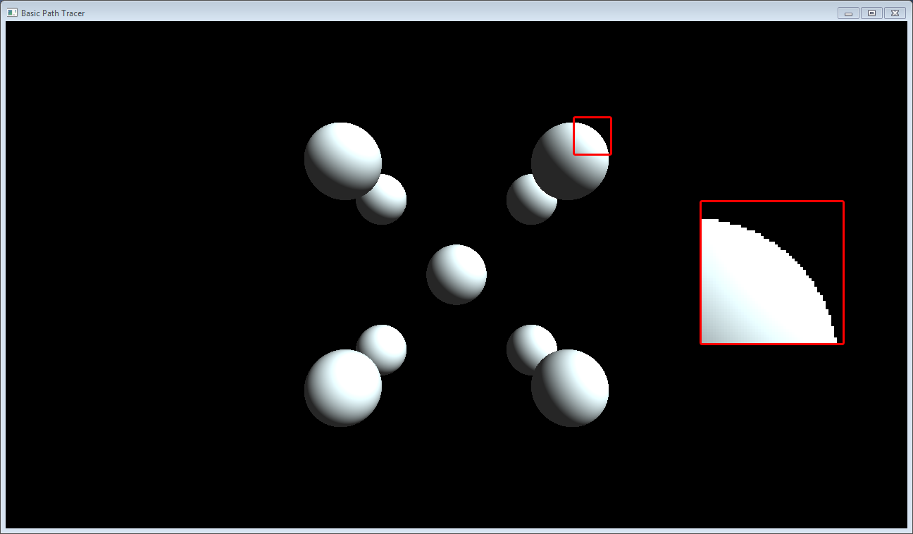
No jitter: Ewwwwwww. Look at all those jaggies......
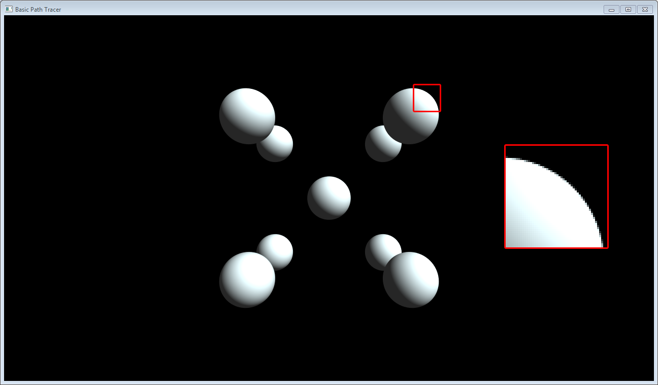
With jitter: Silky smooth :)
Start Bouncing!
float3 pixelColor = make_float3(0.0f, 0.0f, 0.0f);
float3 accumulatedMaterialColor = make_float3(1.0f, 1.0f, 1.0f);

// Bounce the ray around the scene
for (uint bounces = 0; bounces < 10; ++bounces) {
Here we initialize two float3's used to accumulate color as we bounce. I'll cover them in detail below. Then we start a for loop the determines how many times we can bounce around the scene.
Shooting the Scene
// Initialize the intersection variables
float closestIntersection = FLT_MAX;
float3 normal;
Scene::LambertMaterial material;

TestSceneIntersection(ray, sceneObjects, &closestIntersection, &normal, &material);
We initialize the intersection variables and then shoot the ray through the scene.
TestSceneIntersection() loops through each object in the scene and tries to intersect it. If it hits, it tests if the new intersection is closer than the current. If so, it replaces the current intersection with the new one. (And updates the normal / material).
__device__ void TestSceneIntersection(Scene::Ray &ray, Scene::SceneObjects &sceneObjects, float *closestIntersection, float3 *normal, Scene::LambertMaterial *material) {
    // Try to intersect with the planes
    for (uint j = 0; j < sceneObjects.NumPlanes; ++j) {
        // Make a local copy
        Scene::Plane plane = sceneObjects.Planes[j];

        float3 newNormal;
        float intersection = TestRayPlaneIntersection(ray, plane, newNormal);
        if (intersection > 0.0f && intersection < *closestIntersection) {
            *closestIntersection = intersection;
            *normal = newNormal;
            *material = sceneObjects.Materials[plane.MaterialId];
        }
    }

    // Try to intersect with the rectangles;
    for (uint j = 0; j < sceneObjects.NumRectangles; ++j) {
        // Make a local copy
        Scene::Rectangle rectangle = sceneObjects.Rectangles[j];

        float3 newNormal;
        float intersection = TestRayRectangleIntersection(ray, rectangle, newNormal);
        if (intersection > 0.0f && intersection < *closestIntersection) {
            *closestIntersection = intersection;
            *normal = newNormal;
            *material = sceneObjects.Materials[rectangle.MaterialId];
        }
    }

    // Try to intersect with the circles;
    for (uint j = 0; j < sceneObjects.NumCircles; ++j) {
        // Make a local copy
        Scene::Circle circle = sceneObjects.Circles[j];

        float3 newNormal;
        float intersection = TestRayCircleIntersection(ray, circle, newNormal);
        if (intersection > 0.0f && intersection < *closestIntersection) {
            *closestIntersection = intersection;
            *normal = newNormal;
            *material = sceneObjects.Materials[circle.MaterialId];
        }
    }

    // Try to intersect with the spheres;
    for (uint j = 0; j < sceneObjects.NumSpheres; ++j) {
        // Make a local copy
        Scene::Sphere sphere = sceneObjects.Spheres[j];

        float3 newNormal;
        float intersection = TestRaySphereIntersection(ray, sphere, newNormal);
        if (intersection > 0.0f && intersection < *closestIntersection) {
            *closestIntersection = intersection;
            *normal = newNormal;
            *material = sceneObjects.Materials[sphere.MaterialId];
        }
    }
}
I added support for two more intersections since the last post.
Ray-Circle and
Ray-Rectangle. (It actually supports any parallelogram, not just rectangles). The idea for both is to first test intersection with the plane, then test if the intersection point is inside the respective shapes. The code/comments should be self explanatory, but feel free to comment if you have a question.
Direct Hit!!!! Or Perhaps Not....
This is where the true path tracing starts to come in. Once we've traced the ray through the scene, there are 2 outcomes: either we hit something, or we missed.
For real-life materials, light doesn't just bounce off the surface of the material, but rather, it also enters the material itself, bouncing and reflecting off the molecules.
Image from Naty Hoffman's Siggraph 2013 Presentation on Physically Based Shading
As you can image, it would be prohibitively expensive to try to calculate the exact scattering of light within the material. Therefore, a common simplification is to calculate the interaction of light with the surface in two parts: diffuse and specular.
Image from Naty Hoffman's Siggraph 2013 Presentation on Physically Based Shading
The diffuse term represents the refraction, absorption, and scattering of light within the material. It is convenient to ignore entry to exit distance for the diffuse term. Doing so allows us to compute the diffuse lighting at a single point.
The specular term represents the reflected light off the surface, aka, mirror-like reflections.
For now, we're going to assume a material is either a perfect diffuse
Lambertian diffuse material, or a perfect specular mirror in order to keep things simple.
First, let's look at the case where we hit a perfectly diffuse surface lit by a single light source, $L_{\text{i}}$. If we plug that into the Monte Carlo Estimate of the Rendering Equation for a single sample, $\text{k}$, we get:
\[L_{\text{o, k}} = L_e + \frac{L_{\text{i, k}} \: \frac{materialColor_{\text{diffuse}}}{\pi} \: (n \cdot v)}{pdf}\]
where $n$ is the surface normal where we hit, and $v$ is the unit vector pointing from the surface to the light. We use the fact that $\left | \cos \theta \right | \equiv (n \cdot v)$ since both $n$ and $v$ are unit length.
For path tracing, $L_{\text{i}}$ represents the light coming from the
next path. ie:
\[L_{\text{i, k}} = L_{\text{o, k + 1}}\]
It's a classic recursive algorithm. ie:
float3 CalculateColorForRay(Scene::Ray &ray, Scene::SceneObjects &sceneObjects) {
    // Initialize the intersection variables
    float closestIntersection = FLT_MAX;
    float3 normal;
    Scene::LambertMaterial material;

    TestSceneIntersection(ray, sceneObjects, &closestIntersection, &normal, &material);

    // Find out if we hit anything
    if (closestIntersection < FLT_MAX) {
        // We hit an object

        // Shoot a new ray
        ray.Origin = ray.Origin + ray.Direction * closestIntersection;

        if (material.MaterialType == Scene::MATERIAL_TYPE_DIFFUSE) {
            // We hit a diffuse surface
            ray.Direction = CreateNewRayDirection();
        } else if (material.MaterialType == Scene::MATERIAL_TYPE_SPECULAR) {
            // We hit a specular surface
            ray.Direction = reflect(ray.Direction, normal);
        }

        return material.EmmisiveColor + CalculateColorForRay(ray, sceneObjects) * material.MainColor * dot(ray.Direction, normal) * 2.0f /* pdf */;
    } else {
        // We didn't hit anything, return the sky color
        return make_float3(0.846f, 0.933f, 0.949f);
    }
}
Unfortunately for us, the GPU doesn't handle recursion well. In fact, it's forbidden in most, if not all, of the GPU programming languages. That said, since multiplication is both
commutative and
distributive, we can factor out all the $\frac{\frac{materialColor_{\text{diffuse}}}{\pi} \: (n \cdot v)}{pdf}$ terms and turn our path tracing algorithm into a iterative solution:
float3 pixelColor = make_float3(0.0f, 0.0f, 0.0f);
float3 accumulatedMaterialColor = make_float3(1.0f, 1.0f, 1.0f);

// Bounce the ray around the scene
for (uint bounces = 0; bounces < 10; ++bounces) {
    // Initialize the intersection variables
    float closestIntersection = FLT_MAX;
    float3 normal;
    Scene::LambertMaterial material;

    TestSceneIntersection(ray, sceneObjects, &closestIntersection, &normal, &material);

    // Find out if we hit anything
    if (closestIntersection < FLT_MAX) {
        // We hit an object

        // Add the emmisive light
        pixelColor += accumulatedMaterialColor * material.EmmisiveColor;


        // Shoot a new ray

        // Set the origin at the intersection point
        ray.Origin = ray.Origin + ray.Direction * closestIntersection;
        // Offset the origin to prevent self intersection
        ray.Origin += normal * 0.001f;

        // Choose the direction based on the material
        if (material.MaterialType == Scene::MATERIAL_TYPE_DIFFUSE) {
            ray.Direction = CreateUniformDirectionInHemisphere(normal, &randState);

            // Accumulate the diffuse color
            accumulatedMaterialColor *= material.MainColor /* * (1 / PI)  <- this cancels with the PI in the pdf */ * dot(ray.Direction, normal);

            // Divide by the pdf
            accumulatedMaterialColor *= 2.0f; // pdf == 1 / (2 * PI)
        } else if (material.MaterialType == Scene::MATERIAL_TYPE_SPECULAR) {
            ray.Direction = reflect(ray.Direction, normal);

            // Accumulate the specular color
            accumulatedMaterialColor *= material.MainColor;
        }
    } else {
        // We didn't hit anything, return the sky color
        pixelColor += accumulatedMaterialColor * make_float3(0.846f, 0.933f, 0.949f);

        break;
    }
}
The last thing to do is to choose the direction for the next path. For mirror specular reflections, this is as simple as using the
reflect function:
ray.Direction = reflect(ray.Direction, normal);
Since it is a perfect reflection, the probability of the reflection in the chosen direction is 1. ie, $pdf_{\text{specular}} = 1$
However, for diffuse reflections, it's a different story. By definition, the diffuse term can represent any internal reflection. Therefore, the light can come out in any direction within the unit hemisphere defined by the surface normal:
So, we need to randomly pick a direction in the unit hemisphere. For now, we'll use use a uniform distribution of directions. In a later post, we'll explore other distributions.
__device__ float3 CreateUniformDirectionInHemisphere(float3 normal, curandState *randState) {
    // Create a random coordinate in spherical space
    // Then calculate the cartesian equivalent
    float z = curand_uniform(randState);
    float r = sqrt(1.0f - z * z);
    float phi = TWO_PI * curand_uniform(randState);
    float x = cos(phi) * r;
    float y = sin(phi) * r;

    // Find an axis that is not parallel to normal
    float3 majorAxis;
    if (abs(normal.x) < INV_SQRT_THREE) {
        majorAxis = make_float3(1, 0, 0);
    } else if (abs(normal.y) < INV_SQRT_THREE) {
        majorAxis = make_float3(0, 1, 0);
    } else {
        majorAxis = make_float3(0, 0, 1);
    }

    // Use majorAxis to create a coordinate system relative to world space
    float3 u = normalize(cross(majorAxis, normal));
    float3 v = cross(normal, u);
    float3 w = normal;

    // Transform from spherical coordinates to the cartesian coordinates space
    // we just defined above, then use the definition to transform to world space
    return normalize(u * x +
                     v * y +
                     w * z);
}
We use two uniformly distributed random numbers to create a random point in the spherical coordinate system. Then we use some trig to convert to Cartesian coordinates. Finally, we transform the random point from local coordinates (ie, relative to the normal) to world coordinates.
To create the transformation coordinate system, we first find the world axis that is
most perpendicular to the normal by comparing each axis of the normal to $\frac{1}{\sqrt{3}}$. $\frac{1}{\sqrt{3}}$ is significant because it's the length at which all 3 axes are equal (since we know the normal is a unit vector). So if any are less than $\frac{1}{\sqrt{3}}$, there is a good chance that axis is the smallest.
Next, we use the cross product to find an axis that is perpendicular to the normal. And finally, we use the cross product again to find an axis that is perpendicular to both the new axis and the normal.
The $pdf$ for a uniformly distributed direction in a hemisphere is:
\[pdf_{\text{hemi}} = \frac{1}{2 \pi}\]
This corresponds to the
solid angle that the random directions can come from. A hemisphere has a solid angle of $2\pi$ steradians.
Shooting Yourself in the Head
// Russian Roulette
if (bounces > 3) {
    float p = max(accumulatedMaterialColor.x, max(accumulatedMaterialColor.y, accumulatedMaterialColor.z));
    if (curand_uniform(&randState) > p) {
        break;
    }
    accumulatedMaterialColor /= p;
}
During path tracing, we keep bouncing until we miss the scene or exceed the maximum number of bounces. But if the scene is closed and maxBounces is large, we could end up bouncing for a very long time. Remember though, that at each bounce, we accumulate the light attenuation of the material we hit ie:
accumulatedMaterialColor will end up getting closer and closer to zero the more bounces we do. Since
accumulatedMaterialColor ends up being multiplied by the emitted light color, it makes very little sense to keep bouncing after a while, since the result won't add very much to the final pixel color.
However, we can't arbitrarily stop bouncing after
accumulatedMaterialColor goes below a certain threshold, since this would create bias in the Monte Carlo Integration. What we
can do, though, is use a random probability to determine the stopping point, as long as we divide out the $pdf$ of the random sample. This is known as Russian Roulette.
In this implementation, we create a uniform random sample and then compare it against the max component of
accumulatedMaterialColor. If the random sample is greater than the max component then we terminate the tracing. If not, we keep the integration unbiased by dividing by the $pdf$ of our calculation. Since we used a uniform random variable, the $pdf$ is just:
\[pdf = \text{p}\]
Success!
If we whip up a simple scene with a plane and 9 balls we get:
Whooo!! Look at those nice soft shadows! And the color bleeding! Houston, this is our first small step towards a battle-ready photo-realistic GPU renderer.
Let's do another! Obligatory Cornell Box:
One thing to note: since the Cornell box scene has a light with very small surface area in comparison to the surface area of the rest of the scene, the probability that a ray will hit the light is relatively low. Therefore, it takes a
long time to converge. The render above was around 30 minutes. In comparison, the 9 balls scene took about 60 seconds to resolve to an acceptable level.
Closing Words
There we go. Our very own path tracer.
I shall call him Squishy and he shall be mine, and he shall be my Squishy. (I really need to stop watching videos right before writing this blog)
The code for everything in this post is on
GitHub. It's open source under the Apache license, so feel free to use it in your own projects.
As always, feel free to ask questions, make comments, and if you find an error, please let me know.
Happy coding!
-
RichieSams


